15 Data Grouping and Aggregation
15.1 Why Grouping and Aggregation Matter in Data Science
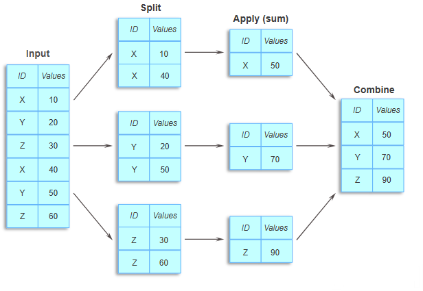
Grouping and aggregation are foundational techniques in data analysis that transform raw data into actionable insights. Here’s why they’re essential:
Data Summarization
Grouping allows you to condense large amounts of data into concise summaries. Aggregation provides statistical summaries (e.g., mean, sum, count), making it easier to understand data trends and characteristics without needing to examine every detail.
Insights Across Categories
Grouping by categories—like regions, demographics, or time periods—lets you analyze patterns within each group. For example:
- Aggregating sales data by region can reveal which areas are performing better.
- Grouping customer data by age group can highlight consumer trends.
- Comparing product performance across different market segments.
Time Series Analysis
In time-series data, grouping by time intervals (e.g., day, month, quarter) allows you to observe trends over time, which is crucial for forecasting, seasonal analysis, and trend detection.
Reducing Data Complexity
By summarizing data at a higher level, you reduce complexity, making it easier to visualize and interpret—especially in large datasets where working with raw data could be overwhelming.
In this chapter, we’ll explore grouping and aggregating using pandas. These methods will help you group and summarize data, making complex analysis comparatively easy.
Throughout this chapter, we’ll use the GDP and Life Expectancy dataset (gdp_lifeExpectancy.csv), which contains information about countries’ GDP per capita and life expectancy over time. This dataset is ideal for demonstrating how grouping can reveal patterns across countries, continents, and years.
Let’s start by importing the necessary libraries and loading the data.
# Import necessary libraries
import pandas as pd
import numpy as np
import seaborn as sns
import matplotlib.pyplot as plt

# Set visualization defaults
sns.set(font_scale=1.5)
%matplotlib inline
# Load the GDP and Life Expectancy dataset
gdp_lifeExp_data = pd.read_csv('./Datasets/gdp_lifeExpectancy.csv')
# Display the first few rows to understand the structure
gdp_lifeExp_data.head()| country | continent | year | lifeExp | pop | gdpPercap | |
|---|---|---|---|---|---|---|
| 0 | Afghanistan | Asia | 1952 | 28.801 | 8425333 | 779.445314 |
| 1 | Afghanistan | Asia | 1957 | 30.332 | 9240934 | 820.853030 |
| 2 | Afghanistan | Asia | 1962 | 31.997 | 10267083 | 853.100710 |
| 3 | Afghanistan | Asia | 1967 | 34.020 | 11537966 | 836.197138 |
| 4 | Afghanistan | Asia | 1972 | 36.088 | 13079460 | 739.981106 |
15.2 Categorical Aggregation
Before diving into advanced grouping operations, it’s important to understand how to aggregate categorical variables. Unlike numerical aggregation (mean, sum, etc.), categorical aggregation focuses on counting frequencies and understanding the distribution of categories.
Categorical aggregation helps answer questions like:
- How many observations belong to each category?
- What’s the distribution across different categories?
- How do two categorical variables relate to each other?
15.2.1 One-way Aggregation: value_counts()
The value_counts() method is the simplest way to count occurrences of each unique value in a categorical column. It returns a Series with categories as the index and their counts as values.
Example: Let’s count how many observations (country-year combinations) we have for each continent.
# Count the number of observations for each continent
continent_counts = gdp_lifeExp_data['continent'].value_counts()
continent_counts
continent
Africa 624
Asia 396
Europe 360
Americas 300
Oceania 24
Name: count, dtype: int64Interpretation: Africa has the most observations (624), while Oceania has the fewest (24). This tells us the dataset has unequal representation across continents.
15.2.1.1 Useful value_counts() Parameters
The value_counts() method has several useful parameters:
normalize=True- Returns proportions instead of countssort=False- Returns results in the order they appear (not sorted by frequency)dropna=False- Includes counts of missing values
Let’s see the proportion of observations in each continent:
# Get proportions instead of counts
continent_proportions = gdp_lifeExp_data['continent'].value_counts(normalize=True)
print("Proportions of observations by continent:")
print(continent_proportions)
print(f"\nAfrica represents {continent_proportions['Africa']:.1%} of all observations")
Proportions of observations by continent:
continent
Africa 0.366197
Asia 0.232394
Europe 0.211268
Americas 0.176056
Oceania 0.014085
Name: proportion, dtype: float64
Africa represents 36.6% of all observations15.2.2 Two-way Aggregation: crosstab()
While value_counts() works for a single categorical variable, crosstab() is used to examine the relationship between two categorical variables. It creates a frequency table (also called a contingency table) showing counts for each combination of categories.
Use case: crosstab() is ideal for:
- Understanding how categories from two variables overlap
- Checking data balance across multiple dimensions
- Creating frequency tables for statistical analysis
The crosstab() method is a special case of a pivot table specifically designed for computing group frequencies (or the size of each group).
15.2.2.1 Basic crosstab() Example
Let’s start with a simple one-way frequency count using crosstab(). While value_counts() is more direct for this purpose, crosstab() can do it too:
# Create a basic crosstab to count observations by continent
# The 'columns' parameter is just a label for the column header
pd.crosstab(gdp_lifeExp_data['continent'], columns='count')| col_0 | count |
|---|---|
| continent | |
| Africa | 624 |
| Americas | 300 |
| Asia | 396 |
| Europe | 360 |
| Oceania | 24 |
15.2.2.2 Two-way Frequency Table
Now let’s create a two-way frequency table to see how observations are distributed across both continent and year. This helps us understand the temporal coverage for each continent.
Adding Margins:
Use the margins=True argument to add row and column totals. The All row and column provide the sum across each dimension.
# Create a two-way frequency table for continent and year
continent_year_table = pd.crosstab(
    gdp_lifeExp_data['continent'],
    gdp_lifeExp_data['year'],
    margins=True
)

# Display the table
continent_year_table| year | 1952 | 1957 | 1962 | 1967 | 1972 | 1977 | 1982 | 1987 | 1992 | 1997 | 2002 | 2007 | All |
|---|---|---|---|---|---|---|---|---|---|---|---|---|---|
| continent | |||||||||||||
| Africa | 52 | 52 | 52 | 52 | 52 | 52 | 52 | 52 | 52 | 52 | 52 | 52 | 624 |
| Americas | 25 | 25 | 25 | 25 | 25 | 25 | 25 | 25 | 25 | 25 | 25 | 25 | 300 |
| Asia | 33 | 33 | 33 | 33 | 33 | 33 | 33 | 33 | 33 | 33 | 33 | 33 | 396 |
| Europe | 30 | 30 | 30 | 30 | 30 | 30 | 30 | 30 | 30 | 30 | 30 | 30 | 360 |
| Oceania | 2 | 2 | 2 | 2 | 2 | 2 | 2 | 2 | 2 | 2 | 2 | 2 | 24 |
| All | 142 | 142 | 142 | 142 | 142 | 142 | 142 | 142 | 142 | 142 | 142 | 142 | 1704 |
Interpretation:
- Each cell shows the count of country-year observations for that continent-year combination
- The
Allcolumn shows total observations per continent (same asvalue_counts()) - The
Allrow shows total observations per year - The bottom-right cell (1704) is the grand total of all observations
This table is useful for:
- Checking if data is representative across all groups
- Identifying any missing years for specific continents
- Understanding the temporal balance of your dataset
15.2.2.3 Using crosstab() with Aggregation Functions
So far, we’ve used crosstab() to count frequencies. However, you can also use it to aggregate numerical values for each category combination by specifying:
values- The numerical column to aggregateaggfunc- The aggregation function to apply (e.g.,mean
,sum
,median
)
This makes crosstab() a powerful tool that combines categorical grouping with numerical aggregation.
Example: Calculate the mean life expectancy for each continent-year combination.
This helps us see how life expectancy has evolved over time across different continents.
# Calculate mean life expectancy for each continent-year combination
mean_lifeExp_table = pd.crosstab(
    gdp_lifeExp_data['continent'],
    gdp_lifeExp_data['year'],
    values=gdp_lifeExp_data['lifeExp'],
    aggfunc='mean'
)

# Round to 1 decimal place for better readability
mean_lifeExp_table = mean_lifeExp_table.round(1)

# Display the table
mean_lifeExp_table| year | 1952 | 1957 | 1962 | 1967 | 1972 | 1977 | 1982 | 1987 | 1992 | 1997 | 2002 | 2007 |
|---|---|---|---|---|---|---|---|---|---|---|---|---|
| continent | ||||||||||||
| Africa | 39.1 | 41.3 | 43.3 | 45.3 | 47.5 | 49.6 | 51.6 | 53.3 | 53.6 | 53.6 | 53.3 | 54.8 |
| Americas | 53.3 | 56.0 | 58.4 | 60.4 | 62.4 | 64.4 | 66.2 | 68.1 | 69.6 | 71.2 | 72.4 | 73.6 |
| Asia | 46.3 | 49.3 | 51.6 | 54.7 | 57.3 | 59.6 | 62.6 | 64.9 | 66.5 | 68.0 | 69.2 | 70.7 |
| Europe | 64.4 | 66.7 | 68.5 | 69.7 | 70.8 | 71.9 | 72.8 | 73.6 | 74.4 | 75.5 | 76.7 | 77.6 |
| Oceania | 69.3 | 70.3 | 71.1 | 71.3 | 71.9 | 72.9 | 74.3 | 75.3 | 76.9 | 78.2 | 79.7 | 80.7 |
Key Insights:
- Life expectancy has generally increased over time across all continents
- Oceania consistently has the highest life expectancy
- Africa has the lowest life expectancy, though it’s improving
- The gap between continents is gradually narrowing over time
While crosstab() is excellent for two-way categorical analysis, groupby() offers significantly more flexibility:
Think of it as a progression:
value_counts()→ Count frequencies for one variablecrosstab()→ Cross-tabulate two categorical variables with optional aggregationgroupby()→ The most flexible and powerful grouping tool for all scenarios
In the next section, we’ll explore groupby() in depth, starting with single-column grouping and gradually building up to more complex operations.
15.3 groupby(): Grouping by a Single Column
The groupby() method allows you to split a DataFrame based on the values in one or more columns, creating groups that can be analyzed separately. Unlike crosstab(), which is optimized for creating cross-tabulation tables, groupby() gives you complete control over how to aggregate, transform, and filter your data.
15.3.1 Syntax of groupby()
DataFrame.groupby(by="column_name")This creates a GroupBy object that represents the grouped data.
15.3.2 Example: Grouping by Continent
Let’s group the life expectancy data by continent. This will allow us to analyze statistics separately for each continent.
# Create a GroupBy object by grouping data by 'continent'
grouped = gdp_lifeExp_data.groupby('continent')

# This logically splits the data into groups based on unique values of 'continent'
# However, the data is not physically split into separate DataFrames
grouped
<pandas.core.groupby.generic.DataFrameGroupBy object at 0x0000014936493FE0>15.3.3 Understanding the GroupBy Object
The groupby() method returns a GroupBy object, not a DataFrame. This object contains information about how the data is grouped, but doesn’t display the groups directly.
# Check the type of the grouped object
type(grouped)pandas.core.groupby.generic.DataFrameGroupByKey Point: The GroupBy object grouped contains the information about how observations are distributed across groups. Each observation has been assigned to a specific group based on the value of continent for that observation. However, the dataset is not physically split into different DataFrames—all observations remain in the same DataFrame gdp_lifeExp_datauntil you apply an aggregation or transformation.
15.3.4 Exploring GroupBy Objects: Attributes and Methods
The GroupBy object has several useful attributes and methods that help you understand and work with your grouped data. Let’s explore the most important ones.
15.3.4.1 keys - Identifying the Grouping Column(s)
The column(s) used to group the data are called keys. You can view the grouping key(s) using the keys attribute.
# View the grouping key(s)
grouped.keys'continent'15.3.4.2 ngroups - Counting the Number of Groups
The ngroups attribute tells you how many unique groups exist based on the grouping key(s).
# Count the number of groups
grouped.ngroups515.3.4.3 groups - Viewing Group Names and Their Members
The groups attribute returns a dictionary where:
- Keys are the group names (unique values of the grouping column)
- Values are the row indices (labels) of observations belonging to each group
# View the group names (keys of the dictionary)
grouped.groups.keys()
dict_keys(['Africa', 'Americas', 'Asia', 'Europe', 'Oceania'])# View the complete groups dictionary (group names and their row indices)
grouped.groups{'Africa': [24, 25, 26, 27, 28, 29, 30, 31, 32, 33, 34, 35, 36, 37, 38, 39, 40, 41, 42, 43, 44, 45, 46, 47, 120, 121, 122, 123, 124, 125, 126, 127, 128, 129, 130, 131, 156, 157, 158, 159, 160, 161, 162, 163, 164, 165, 166, 167, 192, 193, 194, 195, 196, 197, 198, 199, 200, 201, 202, 203, 204, 205, 206, 207, 208, 209, 210, 211, 212, 213, 214, 215, 228, 229, 230, 231, 232, 233, 234, 235, 236, 237, 238, 239, 252, 253, 254, 255, 256, 257, 258, 259, 260, 261, 262, 263, 264, 265, 266, 267, ...], 'Americas': [48, 49, 50, 51, 52, 53, 54, 55, 56, 57, 58, 59, 132, 133, 134, 135, 136, 137, 138, 139, 140, 141, 142, 143, 168, 169, 170, 171, 172, 173, 174, 175, 176, 177, 178, 179, 240, 241, 242, 243, 244, 245, 246, 247, 248, 249, 250, 251, 276, 277, 278, 279, 280, 281, 282, 283, 284, 285, 286, 287, 300, 301, 302, 303, 304, 305, 306, 307, 308, 309, 310, 311, 348, 349, 350, 351, 352, 353, 354, 355, 356, 357, 358, 359, 384, 385, 386, 387, 388, 389, 390, 391, 392, 393, 394, 395, 432, 433, 434, 435, ...], 'Asia': [0, 1, 2, 3, 4, 5, 6, 7, 8, 9, 10, 11, 84, 85, 86, 87, 88, 89, 90, 91, 92, 93, 94, 95, 96, 97, 98, 99, 100, 101, 102, 103, 104, 105, 106, 107, 216, 217, 218, 219, 220, 221, 222, 223, 224, 225, 226, 227, 288, 289, 290, 291, 292, 293, 294, 295, 296, 297, 298, 299, 660, 661, 662, 663, 664, 665, 666, 667, 668, 669, 670, 671, 696, 697, 698, 699, 700, 701, 702, 703, 704, 705, 706, 707, 708, 709, 710, 711, 712, 713, 714, 715, 716, 717, 718, 719, 720, 721, 722, 723, ...], 'Europe': [12, 13, 14, 15, 16, 17, 18, 19, 20, 21, 22, 23, 72, 73, 74, 75, 76, 77, 78, 79, 80, 81, 82, 83, 108, 109, 110, 111, 112, 113, 114, 115, 116, 117, 118, 119, 144, 145, 146, 147, 148, 149, 150, 151, 152, 153, 154, 155, 180, 181, 182, 183, 184, 185, 186, 187, 188, 189, 190, 191, 372, 373, 374, 375, 376, 377, 378, 379, 380, 381, 382, 383, 396, 397, 398, 399, 400, 401, 402, 403, 404, 405, 406, 407, 408, 409, 410, 411, 412, 413, 414, 415, 416, 417, 418, 419, 516, 517, 518, 519, ...], 'Oceania': [60, 61, 62, 63, 64, 65, 66, 67, 68, 69, 70, 71, 1092, 1093, 1094, 1095, 1096, 1097, 1098, 1099, 1100, 1101, 1102, 1103]}You can also access just the row indices (values) for all groups:
# View the row indices for all groups
grouped.groups.values()
dict_values([Index([ 24, 25, 26, 27, 28, 29, 30, 31, 32, 33,
...
1694, 1695, 1696, 1697, 1698, 1699, 1700, 1701, 1702, 1703],
dtype='int64', length=624), Index([ 48, 49, 50, 51, 52, 53, 54, 55, 56, 57,
...
1634, 1635, 1636, 1637, 1638, 1639, 1640, 1641, 1642, 1643],
dtype='int64', length=300), Index([ 0, 1, 2, 3, 4, 5, 6, 7, 8, 9,
...
1670, 1671, 1672, 1673, 1674, 1675, 1676, 1677, 1678, 1679],
dtype='int64', length=396), Index([ 12, 13, 14, 15, 16, 17, 18, 19, 20, 21,
...
1598, 1599, 1600, 1601, 1602, 1603, 1604, 1605, 1606, 1607],
dtype='int64', length=360), Index([ 60, 61, 62, 63, 64, 65, 66, 67, 68, 69, 70, 71,
1092, 1093, 1094, 1095, 1096, 1097, 1098, 1099, 1100, 1101, 1102, 1103],
dtype='int64')])15.3.4.4 size() - Counting Observations per Group
The size() method returns the number of observations in each group. This is useful for understanding the distribution of data across groups.
# Count the number of observations in each continent group
grouped.size()
continent
Africa 624
Americas 300
Asia 396
Europe 360
Oceania 24
dtype: int6415.3.4.5 first() - Viewing the First Element of Each Group
The first() method returns the first non-missing element from each group. This can be useful for quickly inspecting what each group looks like.
# View the first non-missing observation from each continent group
grouped.first()| country | year | lifeExp | pop | gdpPercap | |
|---|---|---|---|---|---|
| continent | |||||
| Africa | Algeria | 1952 | 43.077 | 9279525 | 2449.008185 |
| Americas | Argentina | 1952 | 62.485 | 17876956 | 5911.315053 |
| Asia | Afghanistan | 1952 | 28.801 | 8425333 | 779.445314 |
| Europe | Albania | 1952 | 55.230 | 1282697 | 1601.056136 |
| Oceania | Australia | 1952 | 69.120 | 8691212 | 10039.595640 |
15.3.4.6 get_group() - Extracting Data for a Specific Group
The get_group() method returns all observations belonging to a particular group. This is useful when you want to analyze or visualize a specific group in detail.
# Extract all observations for the 'Asia' continent
grouped.get_group('Asia').head(10)| country | continent | year | lifeExp | pop | gdpPercap | |
|---|---|---|---|---|---|---|
| 0 | Afghanistan | Asia | 1952 | 28.801 | 8425333 | 779.445314 |
| 1 | Afghanistan | Asia | 1957 | 30.332 | 9240934 | 820.853030 |
| 2 | Afghanistan | Asia | 1962 | 31.997 | 10267083 | 853.100710 |
| 3 | Afghanistan | Asia | 1967 | 34.020 | 11537966 | 836.197138 |
| 4 | Afghanistan | Asia | 1972 | 36.088 | 13079460 | 739.981106 |
| 5 | Afghanistan | Asia | 1977 | 38.438 | 14880372 | 786.113360 |
| 6 | Afghanistan | Asia | 1982 | 39.854 | 12881816 | 978.011439 |
| 7 | Afghanistan | Asia | 1987 | 40.822 | 13867957 | 852.395945 |
| 8 | Afghanistan | Asia | 1992 | 41.674 | 16317921 | 649.341395 |
| 9 | Afghanistan | Asia | 1997 | 41.763 | 22227415 | 635.341351 |
15.4 Data Aggregation Within Groups
Once you’ve created a GroupBy object, the real power comes from applying aggregation functions to summarize the data within each group. Aggregation functions compute summary statistics that help you understand patterns and trends across different groups.
15.4.1 Common Aggregation Functions
Below are the most commonly used aggregation functions when working with grouped data in pandas:
| Function | Description | Example Use Case |
|---|---|---|
mean() |
Calculates the average value | Average life expectancy per continent |
sum() |
Computes the total by summing all values | Total population across countries |
min() |
Finds the minimum value | Lowest GDP per capita in each region |
max() |
Finds the maximum value | Highest life expectancy in each year |
count() |
Counts the number of non-null entries | Number of countries per continent |
median() |
Finds the middle value when sorted | Median income across categories |
std() |
Calculates the standard deviation | Variability in GDP within continents |
Each of these functions helps summarize different aspects of your grouped data, making it easier to identify trends, outliers, and patterns.
15.4.2 Example: Calculating Mean Statistics by Country
Let’s find the mean life expectancy, population, and GDP per capita for each country during the period 1952-2007. This will give us a single summary statistic for each country across all years in the dataset.
Approach:
- Remove columns we don’t want to aggregate (
continentandyear) - Group by
country - Calculate the mean for all remaining numeric columns
# Group the data by 'country' and calculate mean statistics
# First, drop columns we don't want to aggregate
grouped_country = gdp_lifeExp_data.drop(['continent', 'year'], axis=1).groupby('country')

# Calculate the mean for all numeric columns (lifeExp, pop, gdpPercap)
country_means = grouped_country.mean()

# Display the results
country_means.head(10)| lifeExp | pop | gdpPercap | |
|---|---|---|---|
| country | |||
| Afghanistan | 37.478833 | 1.582372e+07 | 802.674598 |
| Albania | 68.432917 | 2.580249e+06 | 3255.366633 |
| Algeria | 59.030167 | 1.987541e+07 | 4426.025973 |
| Angola | 37.883500 | 7.309390e+06 | 3607.100529 |
| Argentina | 69.060417 | 2.860224e+07 | 8955.553783 |
| Australia | 74.662917 | 1.464931e+07 | 19980.595634 |
| Austria | 73.103250 | 7.583298e+06 | 20411.916279 |
| Bahrain | 65.605667 | 3.739132e+05 | 18077.663945 |
| Bangladesh | 49.834083 | 9.075540e+07 | 817.558818 |
| Belgium | 73.641750 | 9.725119e+06 | 19900.758072 |
15.4.3 Calculating Other Statistics
We can apply different aggregation functions to understand the variability and spread of data within each group. Let’s calculate the standard deviation to see how much variation exists within each country over time.
# Calculate the standard deviation for each country
country_std = grouped_country.std()

# Display the results
country_std.head(10)| lifeExp | pop | gdpPercap | |
|---|---|---|---|
| country | |||
| Afghanistan | 5.098646 | 7.114583e+06 | 108.202929 |
| Albania | 6.322911 | 8.285855e+05 | 1192.351513 |
| Algeria | 10.340069 | 8.613355e+06 | 1310.337656 |
| Angola | 4.005276 | 2.672281e+06 | 1165.900251 |
| Argentina | 4.186470 | 7.546609e+06 | 1862.583151 |
| Australia | 4.147774 | 3.915203e+06 | 7815.405220 |
| Austria | 4.379838 | 4.376600e+05 | 9655.281488 |
| Bahrain | 8.571871 | 2.108933e+05 | 5415.413364 |
| Bangladesh | 9.028335 | 3.471166e+07 | 235.079648 |
| Belgium | 3.779658 | 5.206359e+05 | 8391.186269 |
Interpretation: Countries with higher standard deviations in lifeExp experienced greater changes in life expectancy over the years, while those with lower standard deviations remained more stable.
You can apply any of the aggregation functions mentioned earlier (min(), max(), count(), median(), etc.) in the same way to compute different statistics for your groups.
15.5 Multiple and Custom Aggregations Using agg()
While applying single aggregation functions like mean() or std() is useful, you’ll often need to:
- Apply multiple aggregation functions simultaneously
- Use custom aggregation functions that aren’t built into pandas
The agg() method of a GroupBy object provides this flexibility.
15.5.1 Multiple Aggregations on a Single Column
When you need to compute several statistics for the same column, pass a list of function names to agg().
Example: Calculate both the mean and standard deviation of GDP per capita for each country.
# Apply multiple aggregation functions to 'gdpPercap' column
gdp_stats = grouped_country['gdpPercap'].agg(['mean', 'std'])

# Sort by mean GDP per capita (descending) and show top 10
gdp_stats.sort_values(by='mean', ascending=False).head(10)| mean | std | |
|---|---|---|
| country | ||
| Kuwait | 65332.910472 | 33882.139536 |
| Switzerland | 27074.334405 | 6886.463308 |
| Norway | 26747.306554 | 13421.947245 |
| United States | 26261.151347 | 9695.058103 |
| Canada | 22410.746340 | 8210.112789 |
| Netherlands | 21748.852208 | 8918.866411 |
| Denmark | 21671.824888 | 8305.077866 |
| Germany | 20556.684433 | 8076.261913 |
| Iceland | 20531.422272 | 9373.245893 |
| Austria | 20411.916279 | 9655.281488 |
15.5.2 Custom Aggregation Functions
In addition to built-in functions, you can create your own custom aggregation functions. This is useful when you need a statistic that isn’t available in pandas.
Example: Calculate the range (max - min) of GDP per capita for each country using a lambda function.
# Calculate the range (max - min) of gdpPercap for each country using a lambda function
gdp_range = grouped_country['gdpPercap'].agg(lambda x: x.max() - x.min())

# Display the results sorted by range (descending)
gdp_range.sort_values(ascending=False).head(10)
country
Kuwait 85404.702920
Singapore 44828.041413
Norway 39261.768450
Hong Kong, China 36670.557461
Ireland 35465.716022
Austria 29989.416208
United States 28961.171010
Iceland 28913.100762
Japan 28439.111713
Netherlands 27856.361462
Name: gdpPercap, dtype: float64# Alternatively, define a named function for better readability
def range_func(x):
"""Calculate the range (max - min) of a series"""
return x.max() - x.min()# Combine built-in functions with custom functions
gdp_complete_stats = grouped_country['gdpPercap'].agg(['mean', 'std', range_func])
# Sort by range and display top 10 countries
gdp_complete_stats.sort_values(by='range_func', ascending=False).head(10)| mean | std | range_func | |
|---|---|---|---|
| country | |||
| Kuwait | 65332.910472 | 33882.139536 | 85404.702920 |
| Singapore | 17425.382267 | 14926.147774 | 44828.041413 |
| Norway | 26747.306554 | 13421.947245 | 39261.768450 |
| Hong Kong, China | 16228.700865 | 12207.329731 | 36670.557461 |
| Ireland | 15758.606238 | 11573.311022 | 35465.716022 |
| Austria | 20411.916279 | 9655.281488 | 29989.416208 |
| United States | 26261.151347 | 9695.058103 | 28961.171010 |
| Iceland | 20531.422272 | 9373.245893 | 28913.100762 |
| Japan | 17750.869984 | 10131.612545 | 28439.111713 |
| Netherlands | 21748.852208 | 8918.866411 | 27856.361462 |
15.5.3 Renaming Aggregated Columns
For better readability and professional reporting, you can rename the columns resulting from aggregation. Pass a list of tuples to agg(), where each tuple contains:
- The new column name (string)
- The aggregation function (string or callable)
Example: Create a summary table with custom column names and include a 90th percentile calculation.
# Apply multiple aggregations with custom column names
gdp_summary = grouped_country['gdpPercap'].agg(
    [('Average', 'mean'),
     ('Standard Deviation', 'std'),
    ('90th Percentile', lambda x: x.quantile(0.9))
    ])

# Sort by 90th percentile and display top 10
gdp_summary.sort_values(by='90th Percentile', ascending=False).head(10)| Average | Standard Deviation | 90th Percentile | |
|---|---|---|---|
| country | |||
| Kuwait | 65332.910472 | 33882.139536 | 109251.315590 |
| Norway | 26747.306554 | 13421.947245 | 44343.894158 |
| United States | 26261.151347 | 9695.058103 | 38764.132898 |
| Singapore | 17425.382267 | 14926.147774 | 35772.742520 |
| Switzerland | 27074.334405 | 6886.463308 | 34246.394240 |
| Netherlands | 21748.852208 | 8918.866411 | 33376.895065 |
| Ireland | 15758.606238 | 11573.311022 | 33121.539164 |
| Canada | 22410.746340 | 8210.112789 | 32891.561152 |
| Saudi Arabia | 20261.743635 | 8754.387440 | 32808.019502 |
| Austria | 20411.916279 | 9655.281488 | 32085.438987 |
15.6 Multiple Aggregations on Multiple Columns
Often, you’ll want to apply the same aggregation functions to several columns simultaneously. This is straightforward with agg().
Example: Calculate the mean and standard deviation of both life expectancy (lifeExp) and population (pop) for each country.
# Apply the same aggregations to multiple columns
multi_column_stats = grouped_country[['lifeExp', 'pop']].agg(['mean', 'std'])

# Sort by mean life expectancy (descending)
multi_column_stats.sort_values(by=('lifeExp', 'mean'), ascending=False).head(10)| lifeExp | pop | |||
|---|---|---|---|---|
| mean | std | mean | std | |
| country | ||||
| Iceland | 76.511417 | 3.026593 | 2.269781e+05 | 4.854168e+04 |
| Sweden | 76.177000 | 3.003990 | 8.220029e+06 | 6.365660e+05 |
| Norway | 75.843000 | 2.423994 | 4.031441e+06 | 4.107955e+05 |
| Netherlands | 75.648500 | 2.486363 | 1.378680e+07 | 2.005631e+06 |
| Switzerland | 75.565083 | 4.011572 | 6.384293e+06 | 8.582009e+05 |
| Canada | 74.902750 | 3.952871 | 2.446297e+07 | 5.940793e+06 |
| Japan | 74.826917 | 6.494629 | 1.117588e+08 | 1.488988e+07 |
| Australia | 74.662917 | 4.147774 | 1.464931e+07 | 3.915203e+06 |
| Denmark | 74.370167 | 2.220111 | 4.994187e+06 | 3.520599e+05 |
| France | 74.348917 | 4.304761 | 5.295256e+07 | 6.086809e+06 |
15.7 Different Aggregations for Different Columns
Sometimes you need to apply different sets of functions to different columns. For this, pass a dictionary to agg() where:
- Keys are column names
- Values are lists of aggregation functions (as strings or callables)
This approach gives you complete control over which statistics are computed for each column.
# Apply different aggregation functions to different columns using a dictionary
varied_stats = grouped_country.agg({
    'gdpPercap': ['mean', 'std'],      # Mean and std for GDP per capita
    'lifeExp': ['median', 'std'],      # Median and std for life expectancy
    'pop': ['max', 'min']              # Max and min for population
})

# Display the first 10 rows
varied_stats.head(10)| gdpPercap | lifeExp | pop | ||||
|---|---|---|---|---|---|---|
| mean | std | median | std | max | min | |
| country | ||||||
| Afghanistan | 802.674598 | 108.202929 | 39.1460 | 5.098646 | 31889923 | 8425333 |
| Albania | 3255.366633 | 1192.351513 | 69.6750 | 6.322911 | 3600523 | 1282697 |
| Algeria | 4426.025973 | 1310.337656 | 59.6910 | 10.340069 | 33333216 | 9279525 |
| Angola | 3607.100529 | 1165.900251 | 39.6945 | 4.005276 | 12420476 | 4232095 |
| Argentina | 8955.553783 | 1862.583151 | 69.2115 | 4.186470 | 40301927 | 17876956 |
| Australia | 19980.595634 | 7815.405220 | 74.1150 | 4.147774 | 20434176 | 8691212 |
| Austria | 20411.916279 | 9655.281488 | 72.6750 | 4.379838 | 8199783 | 6927772 |
| Bahrain | 18077.663945 | 5415.413364 | 67.3225 | 8.571871 | 708573 | 120447 |
| Bangladesh | 817.558818 | 235.079648 | 48.4660 | 9.028335 | 150448339 | 46886859 |
| Belgium | 19900.758072 | 8391.186269 | 73.3650 | 3.779658 | 10392226 | 8730405 |
15.7.1 Combining Dictionary Syntax with Custom Column Names
You can also use the dictionary approach with custom column names by passing tuples as the aggregation values.
Example: For each country, calculate:
- Mean and standard deviation of life expectancy (with custom names)
- Min and max values of GDP per capita
# Apply different functions to different columns with custom names
custom_varied_stats = grouped_country.agg({
    'lifeExp': [('Average', 'mean'),
    ('Standard deviation', 'std')],
    'gdpPercap': ['min', 'max']
})

# Display the first 10 rows
custom_varied_stats.head(10)| lifeExp | gdpPercap | |||
|---|---|---|---|---|
| Average | Standard deviation | min | max | |
| country | ||||
| Afghanistan | 37.478833 | 5.098646 | 635.341351 | 978.011439 |
| Albania | 68.432917 | 6.322911 | 1601.056136 | 5937.029526 |
| Algeria | 59.030167 | 10.340069 | 2449.008185 | 6223.367465 |
| Angola | 37.883500 | 4.005276 | 2277.140884 | 5522.776375 |
| Argentina | 69.060417 | 4.186470 | 5911.315053 | 12779.379640 |
| Australia | 74.662917 | 4.147774 | 10039.595640 | 34435.367440 |
| Austria | 73.103250 | 4.379838 | 6137.076492 | 36126.492700 |
| Bahrain | 65.605667 | 8.571871 | 9867.084765 | 29796.048340 |
| Bangladesh | 49.834083 | 9.028335 | 630.233627 | 1391.253792 |
| Belgium | 73.641750 | 3.779658 | 8343.105127 | 33692.605080 |
15.8 Grouping by Multiple Columns
Above, we demonstrated grouping by a single column, which is useful for summarizing data based on one categorical variable. However, in many cases, we need to group by multiple columns. Grouping by multiple columns allows us to create more detailed summaries by accounting for multiple categorical variables. This approach enables us to analyze data at a finer granularity, revealing insights that might be missed with single-column grouping alone.
15.8.1 Basic Syntax for Grouping by Multiple Columns
Use groupby() with a list of column names to group data by multiple columns.
DataFrame.groupby(by=["col1", "col2"])
Consider the life expectancy dataset, we can group by both country and continent to analyze gdpPercap, lifeExp, and pop trends for each country within each continent, providing a more comprehensive view of the data.
#Grouping by multiple columns
grouped_continent_contry = gdp_lifeExp_data.groupby(['continent', 'country'])[ "lifeExp"].agg(['mean', 'std', 'max', 'min']).sort_values(by = 'mean', ascending = False)grouped_continent_contry| mean | std | max | min | ||
|---|---|---|---|---|---|
| continent | country | ||||
| Europe | Iceland | 76.511417 | 3.026593 | 81.757 | 72.490 |
| Sweden | 76.177000 | 3.003990 | 80.884 | 71.860 | |
| Norway | 75.843000 | 2.423994 | 80.196 | 72.670 | |
| Netherlands | 75.648500 | 2.486363 | 79.762 | 72.130 | |
| Switzerland | 75.565083 | 4.011572 | 81.701 | 69.620 | |
| ... | ... | ... | ... | ... | ... |
| Africa | Mozambique | 40.379500 | 4.599184 | 46.344 | 31.286 |
| Guinea-Bissau | 39.210250 | 4.937369 | 46.388 | 32.500 | |
| Angola | 37.883500 | 4.005276 | 42.731 | 30.015 | |
| Asia | Afghanistan | 37.478833 | 5.098646 | 43.828 | 28.801 |
| Africa | Sierra Leone | 36.769167 | 3.937828 | 42.568 | 30.331 |
142 rows × 4 columns
15.8.2 Understanding Hierarchical (Multi-Level) Indexing
- Grouping by multiple columns creates a hierarchical index (also called a multi-level index).
- This index allows each level (e.g., continent, country) to act as an independent category that can be accessed individually.
In the above output, continent and country form a two-level hierarchical index, allowing us to drill down from continent-level to country-level summaries.
grouped_continent_contry.index.nlevels2# get the first level of the index
grouped_continent_contry.index.levels[0]Index(['Africa', 'Americas', 'Asia', 'Europe', 'Oceania'], dtype='object', name='continent')# get the second level of the index
grouped_continent_contry.index.levels[1]Index(['Afghanistan', 'Albania', 'Algeria', 'Angola', 'Argentina', 'Australia',
'Austria', 'Bahrain', 'Bangladesh', 'Belgium',
...
'Uganda', 'United Kingdom', 'United States', 'Uruguay', 'Venezuela',
'Vietnam', 'West Bank and Gaza', 'Yemen, Rep.', 'Zambia', 'Zimbabwe'],
dtype='object', name='country', length=142)15.8.3 Subsetting Data in a Hierarchical Index
grouped_continent_country is still a DataFrame with hierarchical indexing. You can use .loc[] for subsetting, just as you would with a single-level index.
# get the observations for the 'Americas' continent
grouped_continent_contry.loc['Americas'].head()| mean | std | max | min | |
|---|---|---|---|---|
| country | ||||
| Canada | 74.902750 | 3.952871 | 80.653 | 68.750 |
| United States | 73.478500 | 3.343781 | 78.242 | 68.440 |
| Puerto Rico | 72.739333 | 3.984267 | 78.746 | 64.280 |
| Cuba | 71.045083 | 6.022798 | 78.273 | 59.421 |
| Uruguay | 70.781583 | 3.342937 | 76.384 | 66.071 |
# get the mean life expectancy for the 'Americas' continent
grouped_continent_contry.loc['Americas']['mean'].head()
country
Canada 74.902750
United States 73.478500
Puerto Rico 72.739333
Cuba 71.045083
Uruguay 70.781583
Name: mean, dtype: float64# another way to get the mean life expectancy for the 'Americas' continent
grouped_continent_contry.loc['Americas', 'mean'].head()country
Canada 74.902750
United States 73.478500
Puerto Rico 72.739333
Cuba 71.045083
Uruguay 70.781583
Name: mean, dtype: float64You can use a tuple to access data for specific levels in a multi-level index.
# get the observations for the 'United States' country
grouped_continent_contry.loc[( 'Americas', 'United States')]
mean 73.478500
std 3.343781
max 78.242000
min 68.440000
Name: (Americas, United States), dtype: float64grouped_continent_contry.loc[( 'Americas', 'United States'), ['mean', 'std']]mean 73.478500
std 3.343781
Name: (Americas, United States), dtype: float64gdp_lifeExp_data.columnsIndex(['country', 'continent', 'year', 'lifeExp', 'pop', 'gdpPercap'], dtype='object')Finally, you can use reset_index() to convert the hierarchical index into a regular index, allowing you to apply the standard subsetting and filtering methods covered in previous chapters
grouped_continent_contry.reset_index().head()| continent | country | mean | std | max | min | |
|---|---|---|---|---|---|---|
| 0 | Europe | Iceland | 76.511417 | 3.026593 | 81.757 | 72.49 |
| 1 | Europe | Sweden | 76.177000 | 3.003990 | 80.884 | 71.86 |
| 2 | Europe | Norway | 75.843000 | 2.423994 | 80.196 | 72.67 |
| 3 | Europe | Netherlands | 75.648500 | 2.486363 | 79.762 | 72.13 |
| 4 | Europe | Switzerland | 75.565083 | 4.011572 | 81.701 | 69.62 |
15.8.4 Grouping by multiple columns and aggregating multiple variables
#Grouping by multiple columns
grouped_continent_contry_multi = gdp_lifeExp_data.groupby(['continent', 'country','year'])[ ['lifeExp', 'pop', 'gdpPercap']].agg(['mean', 'max', 'min'])
grouped_continent_contry_multi| lifeExp | pop | gdpPercap | |||||||||
|---|---|---|---|---|---|---|---|---|---|---|---|
| mean | max | min | mean | max | min | mean | max | min | |||
| continent | country | year | |||||||||
| Africa | Algeria | 1952 | 43.077 | 43.077 | 43.077 | 9279525.0 | 9279525 | 9279525 | 2449.008185 | 2449.008185 | 2449.008185 |
| 1957 | 45.685 | 45.685 | 45.685 | 10270856.0 | 10270856 | 10270856 | 3013.976023 | 3013.976023 | 3013.976023 | ||
| 1962 | 48.303 | 48.303 | 48.303 | 11000948.0 | 11000948 | 11000948 | 2550.816880 | 2550.816880 | 2550.816880 | ||
| 1967 | 51.407 | 51.407 | 51.407 | 12760499.0 | 12760499 | 12760499 | 3246.991771 | 3246.991771 | 3246.991771 | ||
| 1972 | 54.518 | 54.518 | 54.518 | 14760787.0 | 14760787 | 14760787 | 4182.663766 | 4182.663766 | 4182.663766 | ||
| ... | ... | ... | ... | ... | ... | ... | ... | ... | ... | ... | ... |
| Oceania | New Zealand | 1987 | 74.320 | 74.320 | 74.320 | 3317166.0 | 3317166 | 3317166 | 19007.191290 | 19007.191290 | 19007.191290 |
| 1992 | 76.330 | 76.330 | 76.330 | 3437674.0 | 3437674 | 3437674 | 18363.324940 | 18363.324940 | 18363.324940 | ||
| 1997 | 77.550 | 77.550 | 77.550 | 3676187.0 | 3676187 | 3676187 | 21050.413770 | 21050.413770 | 21050.413770 | ||
| 2002 | 79.110 | 79.110 | 79.110 | 3908037.0 | 3908037 | 3908037 | 23189.801350 | 23189.801350 | 23189.801350 | ||
| 2007 | 80.204 | 80.204 | 80.204 | 4115771.0 | 4115771 | 4115771 | 25185.009110 | 25185.009110 | 25185.009110 | ||
1704 rows × 9 columns
Breaking Down Grouping and Aggregation
Grouping by Multiple Columns:
In this example, we are grouping the data by three columns:continent,country, andyear. This creates groups based on unique combinations of these columns.Aggregating Multiple Variables:
We apply multiple aggregation functions (mean,std,max, andmin) to multiple variables (lifeExp,pop, andgdpPercap).
This type of operation is commonly referred to as multi-column grouping with multiple aggregations
in pandas. It’s a powerful approach because it allows us to obtain a detailed statistical summary for each combination of grouping columns across several variables.
# its columns are also two levels deep
grouped_continent_contry_multi.columns.nlevels2# pass a tuple to the loc() method to access the values of the multi-level columns with a multi-level index
grouped_continent_contry_multi.loc[('Americas','United States'), ('lifeExp', 'mean')]year
1952 68.440
1957 69.490
1962 70.210
1967 70.760
1972 71.340
1977 73.380
1982 74.650
1987 75.020
1992 76.090
1997 76.810
2002 77.310
2007 78.242
Name: (lifeExp, mean), dtype: float6415.9 Advanced Operations within groups: apply(), transform(), and filter()
15.9.1 Using apply() on groups
The apply() function applies a custom function to each group, allowing for flexible operations. The function can return either a scalar, Series, or DataFrame.
Example: Consider the life expectancy dataset, find the top 3 life expectancy values for each continent
We’ll first define a function that sorts a dataset by decreasing life expectancy and returns the top 3 rows. Then, we’ll apply this function on each group using the apply() method of the GroupBy object.
# Define a function to get the top 3 rows based on life expectancy for each group
def top_3_life_expectancy(group):
    return group.nlargest(3, 'lifeExp')
#Defining the groups in the data
grouped_gdpcapital_data = gdp_lifeExp_data.groupby('continent')Now we’ll use the apply() method to apply the top_3_life_expectancy() function on each group of the object grouped_gdpcapital_data.
# Apply the function to each continent group
top_life_expectancy = gdp_lifeExp_data.groupby('continent')[['continent', 'country', 'year', 'lifeExp', 'gdpPercap']].apply(top_3_life_expectancy).reset_index(drop=True)

# Display the result
top_life_expectancy.head()| continent | country | year | lifeExp | gdpPercap | |
|---|---|---|---|---|---|
| 0 | Africa | Reunion | 2007 | 76.442 | 7670.122558 |
| 1 | Africa | Reunion | 2002 | 75.744 | 6316.165200 |
| 2 | Africa | Reunion | 1997 | 74.772 | 6071.941411 |
| 3 | Americas | Canada | 2007 | 80.653 | 36319.235010 |
| 4 | Americas | Canada | 2002 | 79.770 | 33328.965070 |
The top_3_life_expectancy() function is applied to each group, and the results are concatenated internally with the concat() function. The output therefore has a hierarchical index whose outer level indices are the group keys.
We can also use a lambda function instead of separately defining the function top_3_life_expectancy():
# Use a lambda function to get the top 3 life expectancy values for each continent
top_life_expectancy = (
    gdp_lifeExp_data
    .groupby('continent')[['continent', 'country', 'year', 'lifeExp', 'gdpPercap']]  # Avoid adding group labels in the index
    .apply(lambda x: x.nlargest(3, 'lifeExp'))
    .reset_index(drop=True)
)

# Display the result
top_life_expectancy.head()| continent | country | year | lifeExp | gdpPercap | |
|---|---|---|---|---|---|
| 0 | Africa | Reunion | 2007 | 76.442 | 7670.122558 |
| 1 | Africa | Reunion | 2002 | 75.744 | 6316.165200 |
| 2 | Africa | Reunion | 1997 | 74.772 | 6071.941411 |
| 3 | Americas | Canada | 2007 | 80.653 | 36319.235010 |
| 4 | Americas | Canada | 2002 | 79.770 | 33328.965070 |
15.9.2 Using transform() on Groups
The transform() function applies a function to each group and returns a Series aligned with the original DataFrame’s index. This makes it suitable for adding or modifying columns based on group-level calculations.
Recall that in the data cleaning and preparation chapter, we imputed missing values based on correlated variables in the dataset.
In the example provided, some countries had missing values for GDP per capita. To handle this, we imputed the missing GDP per capita for each country using the average GDP per capita of its corresponding continent.
Now, we’ll explore an alternative approach using groupby() and transform() to perform this imputation.
Let us read the datasets and the function that makes a visualization to compare the imputed values with the actual values.
#Importing data with missing values
gdp_missing_data = pd.read_csv('./Datasets/GDP_missing_data.csv')

#Importing data with all values
gdp_complete_data = pd.read_csv('./Datasets/GDP_complete_data.csv')
# Index of rows with missing values for GDP per capita
null_ind_gdpPC = gdp_missing_data.index[gdp_missing_data.gdpPerCapita.isnull()]
# Define a function to plot and evaluate imputed values vs actual values
def plot_actual_vs_predicted(y, title_suffix=""):
"""
Plot imputed vs actual GDP per capita values and display RMSE.
Parameters:
- y: DataFrame with imputed gdpPerCapita values
- title_suffix: Optional string to add to the plot (e.g., method name)
"""
fig, ax = plt.subplots(figsize=(8, 6))
# Extract actual and imputed values
x = gdp_complete_data.loc[null_ind_gdpPC, 'gdpPerCapita']
y_imputed = y.loc[null_ind_gdpPC, 'gdpPerCapita']
# Create scatter plot
ax.scatter(x, y_imputed, alpha=0.6, s=50)
# Add perfect prediction line (45-degree line)
ax.plot(x, x, color='orange', linewidth=2, label='Perfect imputation')
# Labels and formatting
ax.set_xlabel('Actual GDP per capita', fontsize=14)
ax.set_ylabel('Imputed GDP per capita', fontsize=14)
ax.xaxis.set_major_formatter('${x:,.0f}')
ax.yaxis.set_major_formatter('${x:,.0f}')
ax.tick_params(labelsize=12)
ax.grid(True, alpha=0.3)
ax.legend(fontsize=11)
# Calculate and display RMSE
rmse = np.sqrt(np.mean((y_imputed - x)**2))
# Position text dynamically based on data range
x_pos = x.min() + (x.max() - x.min()) * 0.05
y_pos = y_imputed.max() - (y_imputed.max() - y_imputed.min()) * 0.1
ax.text(x_pos, y_pos, f'RMSE = ${rmse:,.2f}',
fontsize=13, bbox=dict(boxstyle='round', facecolor='wheat', alpha=0.5))
plt.tight_layout()
plt.show()
return rmseApproach 1: Using the `.loc``
# Finding the mean GDP per capita of the continent
avg_gdpPerCapita = gdp_missing_data['gdpPerCapita'].groupby(gdp_missing_data['continent']).mean()

# Creating a copy of missing data to impute missing values
gdp_imputed_data = gdp_missing_data.copy()

# Replacing missing GDP per capita with the mean GDP per capita for the corresponding continent
for cont in avg_gdpPerCapita.index:
    gdp_imputed_data.loc[(gdp_imputed_data.continent==cont) & (gdp_imputed_data.gdpPerCapita.isnull()),
                     'gdpPerCapita'] = avg_gdpPerCapita[cont]

# Plot the actual vs predicted values
plot_actual_vs_predicted(gdp_imputed_data)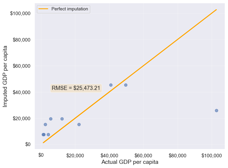
25473.20645170116Approach 2: Using the groupby() and transform() methods.
The transform() function is a powerful tool for filling missing values in grouped data. It allows us to apply a function across each group and align the result back to the original DataFrame, making it perfect for filling missing values based on group statistics.
In this example, we use transform() to impute missing values in the gdpPerCapita column by filling them with the mean gdpPerCapita of each continent:
# Creating a copy of missing data to impute missing values
gdp_imputed_data = gdp_missing_data.copy()

# Grouping data by continent
grouped = gdp_missing_data.groupby('continent')

# Imputing missing values with the mean GDP per capita of the continent
gdp_imputed_data['gdpPerCapita'] = grouped['gdpPerCapita'].transform(lambda x: x.fillna(x.mean()))

# Plot the actual vs predicted values
plot_actual_vs_predicted(gdp_imputed_data)
25473.20645170116Using the transform() function, missing values in gdpPerCapita for each group are filled with the group’s mean gdpPerCapita. This approach is not only more convenient to write but also faster compared to using for loops. While a for loop imputes missing values one group at a time, transform() performs built-in operations (like mean, sum, etc.) in a way that is optimized internally, making it more efficient.
Let’s use apply() instead of transform() with groupby()
Please copy the code below and run it in your notebook:
#Creating a copy of missing data to impute missing values
gdp_imputed_data = gdp_missing_data.copy()

#Grouping data by continent
grouped = gdp_missing_data.groupby('continent')

#Applying the lambda function on the 'gdpPerCapita' column of the groups
gdp_imputed_data['gdpPerCapita'] = grouped['gdpPerCapita'].apply(lambda x: x.fillna(x.mean()))

plot_actual_vs_predicted()
Why we ran into this error? and apply() doesn’t work?
Here’s a deeper look at why apply() doesn’t work as expected here:
15.9.2.1 Behavior of groupby().apply() vs. groupby().transform()
groupby().apply(): This method applies a function to each group and returns the result with a hierarchical (multi-level) index by default. This hierarchical index can make it difficult to align the result back to a single column in the original DataFrame.groupby().transform(): In contrast,transform()is specifically designed to apply a function to each group and return a Series that is aligned with the original DataFrame’s index. This alignment makes it directly compatible for assignment to a new or existing column in the original DataFrame.
15.9.2.2 Why transform() Works for Imputation
When using transform() to fill missing values, it applies the function (e.g., fillna(x.mean())) based on each group’s statistics, such as the mean, while keeping the result aligned with the original DataFrame’s index. This allows for smooth assignment to a column in the DataFrame without any index mismatch issues.
Additionally, transform() applies the function to each element in a group independently and returns a result that has the same shape as the original data, making it ideal for adding or modifying columns.
15.9.3 Using filter() on Groups
The filter() function filters entire groups based on a condition. It evaluates each group and keeps only those that meet the specified criteria.
Example: Keep only the countries where the mean life expectancy is greater than 70
# keep only the continent where the mean life expectancy is greater than 74
gdp_lifeExp_data.groupby('continent').filter(lambda x: x['lifeExp'].mean() > 74)['continent'].unique()
array(['Oceania'], dtype=object)# keep only the country where the mean life expectancy is greater than 74
gdp_lifeExp_data.groupby('country').filter(lambda x: x['lifeExp'].mean() > 74)['country'].unique()array(['Australia', 'Canada', 'Denmark', 'France', 'Iceland', 'Italy',
'Japan', 'Netherlands', 'Norway', 'Spain', 'Sweden', 'Switzerland'],
dtype=object)Using .nunique() get the number of countries that satisfy this condition
gdp_lifeExp_data.groupby('country').filter(lambda x: x['lifeExp'].mean() > 74)['country'].nunique()1215.10 Sampling data by group
If a dataset contains a large number of observations, operating on it can be computationally expensive. Instead, working on a sample of entire observations is a more efficient alterative. The groupby() method combined with apply() can be used for stratified random sampling from a large dataset.
Before taking the random sample, let us find the number of countries in each continent.
gdp_lifeExp_data.continent.value_counts()continent
Africa 624
Asia 396
Europe 360
Americas 300
Oceania 24
Name: count, dtype: int64Let us take a random sample of 650 observations from the entire dataset.
sample_lifeExp_data = gdp_lifeExp_data.sample(650)Now, let us see the number of countries of each continent in our sample.
sample_lifeExp_data.continent.value_counts()continent
Africa 236
Asia 154
Europe 136
Americas 113
Oceania 11
Name: count, dtype: int64Some of the continent have a very low representation in the data. To rectify this, we can take a random sample of 130 observations from each of the 5 continents. In other words, we can take a random sample from each of the continent-based groups.
evenly_sampled_lifeExp_data = gdp_lifeExp_data.groupby('continent').apply(lambda x:x.sample(130, replace=True), include_groups=False)

group_sizes = evenly_sampled_lifeExp_data.groupby(level=0).size()
print(group_sizes)
continent
Africa 130
Americas 130
Asia 130
Europe 130
Oceania 130
dtype: int64The above stratified random sample equally represents all the continent.
15.11 corr(): Correlation by group
The corr() method of the GroupBy object returns the correlation between all pairs of columns within each group.
Example: Find the correlation between lifeExp and gdpPercap for each continent-country level combination.
gdp_lifeExp_data.groupby(['continent','country']).apply(lambda x:x['lifeExp'].corr(x['gdpPercap']), include_groups=False)continent country
Africa Algeria 0.904471
Angola -0.301079
Benin 0.843949
Botswana 0.005597
Burkina Faso 0.881677
...
Europe Switzerland 0.980715
Turkey 0.954455
United Kingdom 0.989893
Oceania Australia 0.986446
New Zealand 0.974493
Length: 142, dtype: float64Life expectancy is closely associated with GDP per capita across most continent-country combinations.
15.12 Independent Study
15.12.1 Practice exercise 1
Read the spotify dataset from spotify_data.csv that contains information about tracks and artists
15.12.1.1
Find the mean and standard deviation of the track popularity for each genre.
15.12.1.2
Create a new categorical column, energy_lvl, with two levels – Low energy
and High energy
– using equal-sized bins based on the track’s energy level. Then, calculate the mean, standard deviation, and 90th percentile of track popularity for each genre and energy level combination
15.12.1.3
Find the mean and standard deviation of track popularity and danceability for each genre and energy level. What insights you can gain from the generated table
15.12.1.4
For each genre and energy level, find the mean and standard deviation of the track popularity, and the minimum and maximum values of loudness.
15.12.1.5
Find the most popular artist from each genre.
15.12.1.6
Filter the first 4 columns of the spotify dataset. Drop duplicate observartions in the resulting dataset using the Pandas DataFrame method drop_duplicates(). Find the top 3 most popular artists for each genre.
15.12.1.7
The spotify dataset has more than 200k observations. It may be expensive to operate with so many observations. Take a random sample of 650 observations to analyze spotify data, such that all genres are equally represented.
15.12.1.8
Find the correlation between danceability and track popularity for each genre-energy level combination.
15.12.1.9
Find the number of observations in each group, where each groups corresponds to a distinct genre-energy lvl combination
15.12.1.10
Find the percentage of observations in each group of the above table.
15.12.1.11
What percentage of unique tracks are contributed by the top 5 artists of each genre?
Hint: Find the top 5 artists based on artist_popularity for each genre. Count the total number of unique tracks (track_name) contributed by these artists. Divide this number by the total number of unique tracks in the data. The nunique() function will be useful.